28 May 2014

Excel with Match Schedule for 2014 FIFA World Cup Soccer Brazil

#17 Excel with Match Schedule for 2014 FIFA World Cup Soccer Brazil

For the upcoming Worldcup Soccer I made 3 Excels with the match-schedule, in 3 formats:
-1: Calendar (see fig.1)
-2: Table, with times of your timezone (see fig.2)
-3: Matrix (see fig.3).

To create these Excels, I used a database-program that I once made (with MS Acces 97...), Match, which I used since 2004 until now to track the UEFA and FIFA soccer championships.
In a next post I'll write more about Match, but if you already want to know something more about it, see this webite:

http://eigersoftware.tripod.com/match.htm

or for the Excel-reports that I created with Match for the UEFA and FIFA soccer championships from 2004 until now:

http://www.scribd.com/eigersoftware


The source for the Excel match-schedules is from the FIFA site:

http://resources.fifa.com/mm/document/tournament/competition/01/52/99/91/2014fwc_matchschedule_wgroups_22042014_en_neutral.pdf

which is in calendar-format (as in fig.1), and shows for every match this information:
- Match-ID
- Teams and 'virtual teams' for final-rounds (e.g. team A1 is winner (rank 1) of group A)
- Group (A-H)
- Date and time (in local (Brazilian) time
- City (stadium)


fig.1a: match schedule in Calendar format, with Location on y-axis
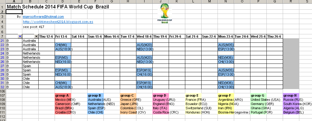

fig.1b: match schedule in Calendar format, with Group/Team on y-axis


fig.2: match schedule in Table format


fig.3: match schedule in Matrix format


Match schedule 1: Calendar format (see fig.1a, 1b)

Fig. 1a:
This schedule is like the schedule on the FIFA site. The only difference is the way I labeled the matches for the final-rounds, e.g.:
- match 49 on Sat.28-6, 1/8-finals, is in cells R13-R14, marked as 'M49', with 'virtual teams' A1 (winner group A) and B2 (runner-up group B)
- match 63 on Sat.12-7 (final for rank 3/4) is in cells AC16-AC17, marked as 'M63', with 'virtual teams' M62R2 (loser semi-final match 62) and M61R2 (loser semi-final match 61)
- match 64 on Sun.13-7 (final for rank 1/2) is in cells AD40-AD41, marked as 'M64', with 'virtual teams' M62R1 (winner semi-final match 62) and M61R1 (winner semi-final match 61)

On the y-axis, the 2 cities marked with '#' (Cuiaba and Manaus) have local time UTC-4, the rest has UTC-3.

Fig.1b:
In this calendar, the y-axis has data from the Group/Team-table in Match (in contrast with fig.1a, which had data from the Location-table). Besides, I put a filter on this column, which in fig.1b is applied to group B, so that the schedule only shows the matches for teams in this group, like the Netherlands and Spain (which were the finalist of the Worldcup in 2010...).

So the Calendar-report is like a pivot-table: In Match you can choose which data (Location or Group/Team) you want on the y-axis. On this website you can find another very nice example how you can present the match-schedule from different viewpoints (location, group, team, date):

http://www.marca.com/deporte/futbol/mundial/calendario/schedule.html

Note: I included this schedule only in Download-Mirror #1.


Match schedule 2: Table format (see fig.2)

Note: The flag-icons come from: 

The table in this report has 2 time-columns: 
-  the local (Brazilian) time, which is (for most cities) UTC-3 or (for 2 cities) UTC-4 (see above). 
- 'your' time, so the time in your time-zone, which is a parameter in the Excel, see cells F3-G3, where you can fill the 'offset' of your timezone in hours (F3) and minutes (G3) with respect to Greenwhich Mean Time (GMT/UTC), e.g.: for CEST (Central European Summer time, which is the time in summer for most European countries), you should fill: 2 (F3) and 0 (G3), which means: UTC + 02:00.

To find your UTC-time, see e.g. : 


So if you live in the CEST-time zone, the 1st match you can see at TV at  22:00 (12-6).

Besides this table, the Excel also has several pivot-tables, which were usefull for me to check if I entered the match-data correctly in my program Match. E.g.: table 2 in sheet 3 shows that in every group the number of matches is 6. Another pivot-table shows the number of matches per city.

And the map with the countries which participate in the Worldcup 2014 (on bottom of sheet) I made with Powermap, see my previous post:

http://worktimesheet2014.blogspot.com.es/2014/05/excel-2013-powermap-and-world-cup-soccer.html


Match schedule 3: Matrix format (see fig.3)

This schedule shows in a compact way for all the matches per group where and when they will be played.

Another (non-Excel) report with the match-schedule generated by Match you can see in fig.4.


fig.4: MS Acces report: match schedule per group


Note 30-5-2014:
The post for Match (my program which generated the Excels in this post) I just finished, see:


Downloads

#Download-Mirror 1 
NB: site has Excel Web-app, if you don't have Excel installed

Table-format:

Calendar-format:

Calendar with Location-view
Matrix-format:


#Download-Mirror 2
(Excels + PDF in 1 zip)


25 May 2014

Pool for betting 2014 World Cup Soccer in Brazil

#16  Pool for betting 2014 World Cup Soccer in Brazil

Note 29-7-2014:
I used this Excel (version 2) for an office-pool, which some small changes. I updated this post to show the results of the office-pool, and also included the final Excel v2 in par. Downloads. I refer to this Excel with V2 and to the original Excel with V1. 

For big sports events like the upcoming 2014 FIFA Worldcup Soccer in Brazil, a lot of people organize with friends or collegues at work a pool to bet who will win the cup. In this post I'll show you how you can do this with Excel, see fig.0 for the end-result (V2)


fig.0: Input office-pool V2


In the table below you can see what you (a gambler) must predict and how many points you can win for each prediction.

Table 1a: Point-system Pool in V1.

V2:
Table 1b: Point-system Pool in V2.

V1:
Points #2 are only calculated when there are more than 1 gamblers with max. points (4), so to tiebreak. The Excel-files with name '*test_Round*' are the result of little demo I made to show how this system calculates the points for 8 gamblers with 8 different predictions, ranging from nothing correct (so 0 points for finalist 1 and 2) to everything correct (finalist 1, 2 winner final and goals winner and loser final all correct). See fig.1 for the end-result of this simulation (row 48, 'Total Points').

V2:
In stead of the finalists (rank 1 and 2) you have to predict which teams end in the top 4 (rank 1-4), and tie-breaking is not the result of the final (goals) but the topscorer of the tournament and his country (so in case no one has predicted the correct topscorer, we look at the country of the top-scorer). In V2 the posibilty of a draw (gamblers with same amount of points) is smaller (that is: the posiblity there is only 1 winner (and not more than 1) is higher). As in V1, a binary point system is used, so that a gambler who predicted correctly e.g. team with rank 1 (16 points) wins from another gambler who predicted correctly the teams with rank 2,3 and 4, but not team with rank 1 (8+4+2=14 points).
In V2, phase 2 is to tie-break in case there are more than 1 gamblers with the same amount of points (no necesary the max. amount of points like in V1)


Fig.1: simulation WorldCup-pool with 8 gamblers, with result after final

Suppose after the Group-round (1), it appears nobody has predicted any of the teams who go to the next round (2) (1/8 finals) correctly (or in other words: all the teams which the gamblers predicted as finalists are eliminitad after round 1), you could say the game is over. But in stead, you could also give everybody a new possibility, so every gambler could give his new predictions (before the start of round 2).

How to use this Excel?
The idea is that it is used by 2 types of users:
- gamblers, who fill in their predictions
-administrator, who checks the gamblers input, and updates the Excel after every round with the results.
NB: WorldCup has 1 Group/Qualification-round and 4 final-rounds: 1/8 finals,  1/4 finals, 1/2 finals, final. (I exclude the match for place/rank 3-4, because for this pool it is not relevant).

How can they do this in the Excel:

* Gambler:
He must fill a '1' and '2' in his column (F7:F38 for gambler G1) on the row of the team he predicts will play the final and win (rank 1) or lose (rank2) and also his predicton of the result of the final (F40: goals winner, F41: goals loser)

* Admin:

- After gamblers completed their input:
Admin. Must check if on row 39 and 41 in the columns with the gambler-input (right to the word 'CHECK') there are no red-cells, only green cells (sum of forecast of teams with rank 1 and 2 must be 3).

- Before every round:
 Admin must fill in cel C3 round-nr: 32 (Group-Qualifications), 16 (1/8 finals), 8 (1/4 finals), 4 (1/2 finals), 2 (final). This round-number should be copied also into column (C7:C38) for each team which is still in the competition and for each eliminated team he should fill a '0'. The total number of teams which are still in the competition you can see in C4, which must be the same as cell C3, round-nr. And if there is a difference (between C3 and C4), you can see it in cell E4 (red if error, green if OK).
In the demo-files (name *test*), I copied the result of every round in a file which name ends with a number which indicates who many teams are in that round, so for the Group-round (with 32 teams), that is 32, for round 2 (1/8 finals) that is 16 ('best of 16) (see fig.2) etc.

- For final:
 Admin. must fill a '1' and '2' in column D7:D38 on the row of the team which will play the final and win (rank 1) or lose (rank2) and also the result of the final (D40: goals winner, D41: goals loser).

Cells where user must input a value (column D for admin, columns F, G etc. for gambler G1, G2 etc) have these data-validations:

- F7: Forecast result, check: allowed values: 1, 2 (for rank 1 and 2, winner and loser of final)

- F39: total forecast result rank 1 and 2 must be 3, manual check (conditional formatting: red = error, green = OK)

- F41: Goals loser, check: Goals loser < Goals winner (F40) (value between 0 and =F40-1)

fig.2: competition in round 2 (1/8 finals, 'best of 16') in simulation V1

In the demo/simulation you can e.g. see:
- Gambler G1 forecasted MEX and CMR are the finalists (cells F7,F8) with rank 1 (winner) and 2 (loser) and with result MEX-CMR: 1-0 (cell F40, F41 in see fig.1)
- Gambler G2 has after round 1 has been played (so at the start of round 2 (1/8 finals) only 1 team which is still in the competition (cell G45 is orange): his forecast for rank 1 and 2 where ESP and FRA, and after round 1, FRA has been eliminitad (cell C23 has value 0) and ESP is in the next round (best of 16) (cell C13 has value 16), see fig.2.
- After the final has been played, gambler G1 had none of its 2 teams which he predicted as finalist correct (cell F45 is red), see fig.1
- After the final has been played, there were 4 gamblers with the maximum number of points (4): G5, G6, G7, G8, and G8 is the winner after the tiebreak, with 7 points, see cell M48 fig.1

The Excel has also a statistic (graphic): Total of betts for rank 1 (winner final) and rank 2 (loser final) per team, see fig.3.

fig.3: Statistics betts in simulation V1

Well, I hope it is clear how this Excel works and that you can use it for your World-Cup pool.


Note 29-7-2014: Results my office-pool:
In the office-pool, there were 12 participants. In fig.4 you can see their predictions for the 32 teams (before start worldcup) and in fig.5 the end-result for the top 4 teams. As you can see, there was only 1 gambler who predicted that the Netherlands would end in the top 4 and it wasn´t me.. but SER7, who in the end also won the pool.


fig.4: predictions before start in V2

fig.5: predictions after end in V2


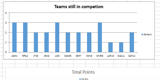
After every phase of the worldcup, I updated column C with 0 o N (16, 8, 4,..) if a team did or did no pass to the next round, and a graphic showed how many teams of each gambler´s prediction were still in the competition (not eliminated), see fig. 6 for result at the end of the worldcup.


fig.6: total teams still in competition at end worldcup (so who ended in top 4)


And the end-result (total points per gambler) was:

fig.7: total points per gambler

As you can see, there were 3 potential winners, so gamblers with the same amount of points (17 of 32) (all 3 had predicted Germany as winner and 1 other team in top 4 although not with the correct rank), also after the tie-break (none of them had the topscorer or his country correct), so we decided to add 1 extra rule: the winner is the one whose prediction of the topscorer is the one with the highest number of goals, and that made SER7 the final winner, which in my opinion he deserved because as I said before, he was the only one who predicted that the Netherlands would end in the top 4.

How to win next time the office-pool for the Worldcup?

*1: Know your ´classics´:
Football is a simple game. Twenty-two men chase a ball for 90 minutes and at the end, the Germans always win. - Gary Lineker

see:
http://www.brainyquote.com/quotes/quotes/g/garylineke422219.html

*2: Get a Windows smartphone:
It´s voice-assistent Cortana predicted 15 of the 16 teams in the elimination-phases (1/8 final until final) correctly, using Big Data techniques (e.g. using dat from prediction-markets), so it is the sucesor of octopus Paul of the 2010 Worldup. See:

http://www.maximumpc.com/microsofts_cortana_voice_assistant_correctly_predicts_world_cup_winner150

*3: Use a more scientific approach, e.g. use game-theory, see e.g. :

http://www.minyanville.com/special-features/sports-business/articles/march-madness-final-four-game-theory/2/27/2012/id/39600


Downloads

#Mirror 1: 

V1: 1 file (without demo)

11 May 2014

Excel 2013, PowerMap and World Cup Soccer

#15  Excel 2013, PowerMap and 2014 World Cup Soccer 

NB: This post has 2 Excel-files (embedded in 1 zip), see ‘Downloads’ at bottom of page. To be able to open these files, you must have Excel 2013 with the Power-BI add-ins installed.


With the 2014 FIFA Worldcup coming closer, I thought it might be interesting to use this event to show the Excel add-in PowerMap,  a component of the Power-BI suite for Excel 2013 which I didn´t show yet in my previous post about Excel and Business Intelligence (BI), see:

http://worktimesheet2014.blogspot.com.es/2014/05/excel-2013-and-business-intelligence.html

As I explained in part 2 of that post, in Excel 2013 you can use PowerView to visualize geospatial data in a map. But with PowerMap you can do much more then that, as you´ll see in this post.

PART 1:

Excel: WorldCupHistory.xlsx

First a little bit of history of the World Cup Soccer. In this Excel, you can see which teams reached the top four (how often did the team end at position 1 to 4) and their final ranking in the tournament (so 1 to 4), for which I used PowerQuery with option 'select from Web', to import the table with this data from:

http://en.wikipedia.org/wiki/FIFA_World_Cup

Then I edited this table a bit, to end up with the table in PowerPivot as you can see in fig.1  (note the column 'Continent' has corresponding datacategory).

fig.1 table in PowerPivot


Then I created in a new sheet in Excel a PowerView report with a map and the winners of all World Cups (so the ones who got the title 'World Campion'), and how often they won, which determines the size of the dot on the map, see fig.2. Note that in Filter 'Titles' value '0' is un-checked (and values '1' to '5' checked), so that the 2 elements in the report (map and table) only show countries which have won 1 or more times the World Cup.

fig.2: PowerView with map

And the last step was to create a simular report with PowerMap, see fig.3.
fig.3: PowerMap

For this report, I chose the options 'Globe (there is also a 'flat-map' variant, see part 2 of this post) and 'bar-charts' (other options are 'dots' or 'regions', see part 2). As you can see in the bottom-left corner, the Bing-Map is used for this, so you must be connected to the web.
NB: the PowerMap-report is stored in Excel in sheet-3, although you don´t directly see it. First, you must activate the COM-addin for PowerMap, see menu File > Options), and then in sheet-3 you must click in menu Insert > PowerMap, and then apears the 'tour' which I created). PowerMap is still in 'preview-version', I suppose Microsoft solves this before the final release.


PART 2:

Excel: WorldCup2014Countries.xlsx

This Excel has a table with the 32 countries which qualified for the 2014 World Cup in Brazil, see e.g.:

http://prosoccertalk.nbcsports.com/2013/11/20/2014-fifa-world-cup-countries-qualified-for-teams-draw-date/

Note that this table is what they call in BI-terms a 'factless fact-table', that is: it has only dimension-columns (type char) and no measures (type number). I could have added a dummy-measure 'counter' which always has value '1', but it is not necessary.
In fig.4 and 5 you can see the reports in PowerView and PowerMap, the last one with options 'Region' (to color the 32 countries) and 'flat map', and if you change this to 'Globe', it shows a nice animated transition from Map to Globe.

fig.4: PowerView

fig.5: PowerMap


For more information about PowerMap, see e.g.:

http://www.databasejournal.com/sqletc/getting-started-with-microsoft-power-map-for-excel.html


Downloads

https://drive.google.com/file/d/0BywxxSJoaUYxdF9HYVAtZ3pLcWs/edit?usp=sharing

7 May 2014

Excel 2013 and Business Intelligence

#14  Excel 2013 and Business Intelligence

NB: This post has 3 Excel-files (embedded in 1 zip), see ‘Downloads’ at bottom of page. To be able to open these files, you must have Excel 2013 with the Power-BI add-ins installed.

Recently I followed a very interesting course about Business intelligence (BI) with MS SQL Server 2012, Analysis Services 2012 and MS Excel 2013. Because this blog is about Excel,  I´ll tell in this post something about Excel 2013 and it's BI-features.

The teacher of this course, who has a blog about BI, see:

www.amby.net

said: “Microsoft wouldn’t be Microsoft without Excel”, meaning that Excel is probably Microsoft's most used product. And with Excel 2013, and it´s 'Power-BI' add-ins like PowerPivot, PowerQuery and PowerView, Microsoft  wants to provide 'self-service business intelligence' (so for business-users), to increase even more the use of Excel.

To start, a definition of BI, from:

http://en.wikipedia.org/wiki/Business_intelligence

Business intelligence (BI) is a set of theories, methodologies, architectures, and technologies that transform raw data into meaningful and useful information for business purposes.

An example of BI with Excel is e.g. a spreadsheet which has all the sales-data of a big international company and then by applying pivot-tables and pitvot-charts, this data can be summarized and presented in a way the general salesmanager can see easily how the business is going, e.g.  the top 10 of most sold products, or the sales per country.


* PART 1

Excel: Skating_XL_PP_Query10_XL13C_v2.xlsx

In this part I´ll use the same database as in the previous post, see:

http://worktimesheet2014.blogspot.com/2014/04/excel-and-relational-databases.html

So first I link my Excel to the Excel-file with the Skating-database (C:\Temp\Skating_DB_XL.xlsx, see 'Downloads' in my previous post), by creating the connection, see fig.1.

fig.1: Connection (relational) database


Then I add the linked-tables in PowerPivot, into a 'tabular model', which is the data-source I'll use from now on to create pivot-tables etc, see fig.2-4.


fig.2: Connection PowerPivot


fig.3 PowerPivot datamodel


fig.4 PowerPivot datamodel: relations


With the Skating-database (3 tables: Race, Skater, Team) imported in the datamodel in PowerPivot, I now can use DAX-formulas (Data Analysis Expressions), which are like ‘normal’ Excel-formulas, except that they work on (rows and columns of) tables (not on cells). For more details about DAX, see e.g.:

http://office.microsoft.com/en-us/excel-help/data-analysis-expressions-dax-in-power-pivot-HA102836919.aspx

2 Examples of DAX-formulas:

*1: Column: Category_MW (Man/Women) = LEFT(T_Race[Race];1), see fig.5. Result: M/W.

*2: Total distinct races  = DISTINCT_Distance:=DISTINCTCOUNT([Distance]), see fig.6. Result: 6.
NB: for this total, we only look at distance, so disregarding gender, so M500 = W500 (race:  men/women over distance 500 meter)

fig.5 DAX-formula


fig.6 DAX-formula


Leaving the PowerPivot-window, you can see in Excel 3 pivot-tables:

*1: Number of skaters per distance (race), with slicer (filter): Gender (Men/Women), see fig.7

*2: Number of skaters per distance (race) X Gender (Men/Women), see fig.8

*3: Medal-total (ranking 1,2,3: gold/silver/bronze) per skater and Gender (Men/Women), see fig.9.

fig.7: Pivot-table 1

fig.8: Pivot-table 2

fig.9: Pivot-table 3


Besides the pivot-tables, the Excel also has a report in PowerView, see sheet-1 and fig.10 for an example. This report has several elements:

* on the top-right, all tables and fields (including the calculated-fields like ‘distinct Distance’) of the database (from the PowerPivot-datamodel, see above)

* the tables in the report (‘Ranking per Skatername’ and ‘Team/Skater-name’ and ‘distinct Distance’)

* filters  (e.g. ‘Gender’ and bar with 1 value per race ‘M1000, M10.000 etc’) which work on the tables, so they make the report ‘interactive’

In fig.10 you can see that:
- in race M1000 (Men 1000 meter) (see slicer), there were 4 (Dutch) skaters participating, and Groothuis won this race (table 1).
- because filter Gender = ’M' (Men), table 2 (Team/Skater-name) shows only the men (not women) in the teams, and the number of races (distinct distance) for men is 5.

fig.10 Report in PowerView


* PART 2

Excel: Skating_PowerviewMap_v3.xlsx

In this Excel you can see how in Excel 2013 with PowerView you can visualize geospatial data in a map.
I created a table in in Excel with the top 10 countries of the medal-ranking from Wintergames 2014, which I copied from:

http://en.wikipedia.org/wiki/2014_Winter_Olympics_medal_table

and I added an extra column, 'Continent', and this table I imported in a 'tabular model' in PowerPivot, see fig.11.

fig.11: datamodel in PowerPivot


After that I enhanced this model by specifying the correct Data Category (in menu Advanced) for the 'Continent' and 'NOC' (Country) fields.  And then when you return to Excel and want to create a report for this data in PowerView, you see that these geographic-columns are marked with a Globe-icon. The maps used by PowerView are those from MS Bing Maps, so you should be 'online' when you want to create a report with maps. The final result you can see in fig.12-13, which show in this case the number of golden medals won per continent and country, with a dot. So you can see easily (by the size of the dot) that in Europe the countries in the North did better then in the South or that a small country like the Netherlands did better then a big country like France.
For more info about the use of Excel and  Maps, see e.g.:

http://www.sqljason.com/2012/07/creating-maps-in-excel-2013-using-power.html

fig.12: PowerView with Bing-Map

fig.13: PowerView with Bing-Map


* PART 3

Excel: WebDB_v2.xlsx

With Excel 2013 and add-in PowerQuery, you have a lot of possibilities to connect to external data and the Excel in this part shows how you can import a table from the Web, in this case I used the 'Overall top goalscorers' table  from:

http://en.wikipedia.org/wiki/UEFA_European_Football_Championship

see fig.14
fig.14 Website with topscorers-table to import in Excel

and for the result, see fig.15-16.

fig.15 topscorers-table import by PowerQuery


fig.16 topscorers-table import by PowerQuery


Note 11-5-2014: Today I created a new post about Excel 2013 and PowerMap (another add-in of the Power-BI suite), with an example for 2014 FIFA World Cup Soccer, see:

http://worktimesheet2014.blogspot.com.es/2014/05/excel-2013-powermap-and-world-cup-soccer.html

Downloads


29 Apr 2014

Excel and relational databases


#13  Excel and relational databases

NB: This post has some files (embedded in 1 zip), see ‘Downloads’ at bottom of page.

In my previous post:
I showed how you can calculate the medal-totals grouped by team, and I also said that this calculation could be much simpler in SQL, the language used in relational databases, like e.g. MS Access. In this post I´ll show you how you can do this in MS Excel, so in a spreadsheet-program. This is useful for those who don´t have an MS Office-version which includes MS Access.

The general idea is to split the application in 2 layers (2 Excel-files): the database-layer and the client-layer, like in a client/server-application.
The database has data about skaters, races and teams. Each type of data is put in it´s own table and between the tables exist relations as you can see in fig.1, e.g.: a team consists of 1 or more skaters and a skater participates in 1 or more races. The tables are linked by their primary keys (PK) and foreign keys (FK), columns which end with ID, e.g. TeamID (PK of table Team and FK of table Skater).


fig.1: Tables in database


The data in these tables you can see in fig.2 and file Skating_DB_XL.xlsx, which is an Excel-workbook with 3 worksheets, one for each table.

NB: I also made this database in MS Access for illustration-purposes, see fig.3 and file Skating_DB_AC.accdb 

fig.2: Excel-file with database

fig.3 Access-file with database


To be able to use these 3 tables in this Excel-file (´database-layer’) in another Excel-file (the ‘client-layer’), you must create a ‘Range’ for each table, see fig.4 and these sites how to do it:


fig.4: Named Ranges for tables in database


In the Excel with the client-layer, you now must create a connection to the Excel with the database-layer, which is stored in a dqy-file (Excel ODBC Query), see these sites how to do this:


With the connection to the database created, you now can use Excel Query to create your queries to the database,  using the Query Wizard (see fig. 5-6) or hand-written SQL (see fig.7 etc.)

fig.5: Excel Query

fig.6: Excel Query with result


Some examples of database queries in SQL:

* Example 1

File: Skating_XL_Query2b.xlsx, Skating_XL_Query2.dqy

Query: ranking for all skaters in top 3 and pivot-table

SQL:
SELECT 
 T_Race.SkaterID,
T_Skater.Gender, T_Skater.SkaterName,
T_Team.TeamID, T_Team.Trainer, T_Team.TeamName,
 T_Race.Race, T_Race.Ranking
FROM `C:\Temp\Skating_DB_XL.xlsx`.T_Race T_Race,
`C:\Temp\Skating_DB_XL.xlsx`.T_Skater T_Skater,
`C:\Temp\Skating_DB_XL.xlsx`.T_Team T_Team
WHERE T_Race.SkaterID = T_Skater.SkaterID
AND T_Skater.TeamID = T_Team.TeamID
AND T_Race.Ranking <=3

fig.7: Result query


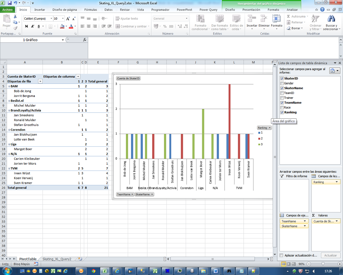
fig.8: pivot table based on result query (fig.7)


*Example 2

Files: Skating_XL_QueryXL_6b.xlsx, Skating_XL_Query6.dqy

Query: medal-total per team

SQL:

SELECT
 Sum(IIF(T_Race.Ranking=1,1,0)) AS 'Total_Gold',
Sum(IIF(T_Race.Ranking=2,1,0)) AS 'Total_Siver',
Sum(IIF(T_Race.Ranking=3,1,0)) AS 'Total_Bronze', Sum(IIF(T_Race.Ranking=1,1,0))+Sum(IIF(T_Race.Ranking=2,1,0))+Sum(IIF(T_Race.Ranking=3,1,0)) AS 'Total',
 T_Team.TeamName
FROM `C:\Temp\Skating_DB_XL.xlsx`.T_Race T_Race,
`C:\Temp\Skating_DB_XL.xlsx`.T_Skater T_Skater,
`C:\Temp\Skating_DB_XL.xlsx`.T_Team T_Team
WHERE T_Race.SkaterID = T_Skater.SkaterID
AND T_Skater.TeamID = T_Team.TeamID
AND ((T_Race.Ranking<=3))
GROUP BY T_Team.TeamName
ORDER BY Sum(IIF(T_Race.Ranking=1,1,0)) DESC, Sum(IIF(T_Race.Ranking=2,1,0)) DESC,  Sum(IIF(T_Race.Ranking=3,1,0)) DESC, T_Team.TeamName


fig.9: Result query


Note 7-5-2014:
I wrote a new post with more examples on the Skating-database in this post, using PowerPivot and PowerView, see:

http://worktimesheet2014.blogspot.com.es/2014/05/excel-2013-and-business-intelligence.html


Download-mirror:


26 Feb 2014

Rankings Dutch skaters in Wintergames Sochi 2014

#12  Rankings Dutch skaters in Wintergames Sochi 2014

Note 28-2-2014
I updated the Excel (see downloads) and this post, see part 3.


Part 1/3 (26-2-2014)

Toyday my last post dedicated to the Wintergames in Sochi 2014. This time I made an Excel (see fig.1) with the results (rankings) of all Dutch long-track skaters (so I excluded the short-track skaters and the team pursuit) of TeamNL. You did a great job at these Games and I congratulate all of you with your results, whether it was gold, silver bronze or a new PR.

To collect all rankings, I used this (Dutch) website:

http://www.schaatsen.nl/sotsji-2014/langebaan

which links to this one:
http://live.isuresults.eu/2013-2014/sochi

and if you click in the ranking-table on the name of a skater, it opens this website (and shows details about the skater).

To highlight the medal-winners, I color-coded rankings 1, 2 and 3 (green, orange, red), using Conditional Formatting. The tables with the medal-totals are calculated with the COUNTIF-formula, see e.g. :
http://www.techonthenet.com/excel/formulas/countif.php

So the Netherlands won 21 medals in longtrack (individual) skating, and 3 more in other disciples, which is a new record. Of course, every person who became a olympic champion has delivered a great performance and deserved to get the Dutch 'knighthood' title, which the Dutch king gave to them the other day (see fig.2), but in case the king could only give one title, I´d say to him to give it to Stefan Groothuis, who after having overcome a very difficult time and a bad start in Sochi (he fell in the 500m), won the 1000m, very impressive!


                                             Fig.1: Ranking Dutch skaters in races at Olympic Wintergames 2014 Sochi


Fig.2: Dutch Skaters with King Willem Alexander and Queen Maxima,
source:


Part 2/3 (27-2-2014)

Today someone asked me about the order of the skaters in the ranking-table. The order doesn´t mean anything, it´s just how the skaters were ordered on this (Dutch) website::

http://www.schaatsen.nl/sotsji-2014/langebaan.

But the question gave me an idea: to order the skaters based on the number of medals they won, in the same way as the countries were ordered at the end of the Games (with the Netherlands at 5th place), see:

http://www.sochi2014.com/en/medals

So: nr.1 is the one who won the most gold medals, and if this is equal for 2 countries/skaters you look who won the the most silver medeals and if this is also equal you look who won the most bronze medals.
So I made a new table in my Excel (sheet 2, see fig.3), copying the table of sheet 1, but just the part with the skaters and their medal-totals for gold/silver/bronze, and then I did a multi-column ordering on this table, see:

http://office.microsoft.com/en-us/excel-help/sort-a-table-HA103993978.aspx#_Toc354843384

To get the ranking-nr (1st column), I added 4 columns (purple) to calculate the difference in the gold/silver/bronze total with the previous skater in the ranking-table, and if this is 0 for all 3 columns, it means the skater has the same ranking as the previous skater.To do this, I used a conditional formula for the 4th purple column:

Ranking_Diff =IF(AND([@[Gold_Diff]]=0;AND([@[Silver_Diff]]=0;[@[Bronze_Diff]]=0));0;1)

see:

http://office.microsoft.com/en-us/excel-help/create-conditional-formulas-HP005251012.aspx

As you can see in fig.3, Ireen Wüst was the most succesfull Dutch skater (and as I said earlier, my Excel only includes the individual long-track competitions (so I excluded short-track and team pursuit, and in the last, Wüst won another gold medal). After these Games, Wüst  is the most succesfull Dutch olympic athlete (so of all olympic sports) ever, see this (Dutch) website::

http://nos.nl/os2014/artikel/614977-wust-beste-nederlandse-olympier.html

And she can even improve her 'score' because she said she will be there at the next Wintergames..


Part 3/3 (28-2-2014)

Besides several skaters, also 2 trainers were given the knighthood title, Gerard Kemkers (of team TVM) and Jac Orie (of team BrandLoyalty/Activia), and they deserve it.
NB: Most of the Dutch skaters train in professional teams, which have the name of their sponsor, only some skaters are independant, so without a team. For more details about the Dutch skaters and teams, see this (Dutch) website:

http://nos.nl/artikel/564722-overzicht-schaatsploegen-20132014.html

I wanted to compare the results of the teams (coaches), so I added to the table in worksheet 2 a colum 'team' (team-ID I should say, no team-name, to save space in the table) and I created a new table with the teams in which I count the total of gold/silver/medals (in the same way as I did for the skaters) with a formula like this (for the total of golden medals for team TVM):

=IF(D4="TVM";E4;0) + IF(D5="TVM";E5;0) + IF(D6="TVM";E6;0) + IF(D7="TVM";E7;0) + IF(D8="TVM";E8;0) + IF(D9="TVM";E9;0) + IF(D10="TVM";E10;0) + IF(D11="TVM";E11;0) + IF(D12="TVM";E12;0) + IF(D13="TVM";E13;0) + IF(D14="TVM";E14;0) + IF(D15="TVM";E15;0) + IF(D16="TVM";E16;0) + IF(D17="TVM";E17;0) + IF(D18="TVM";E18;0) + IF(D19="TVM";E19;0) + IF(D20="TVM";E20;0) + IF(D21="TVM";E21;0) + IF(D22="TVM";E22;0) + IF(D23="TVM";E23;0)

So this formula loops through all rows with the skaters and if the skater is of team TVM, it includes this skaters golden medal-total into the TVM-team´s golden medal-total. For the result, see fig.3, which shows that team TVM, with trainer Kemkers, had the best performance, with a total of 7 medals.

Maybe some of you think this is a very inefficient way to calculate the team-rankings if you compare it how you could do this in a relational database with count-queries, and this is true. Maybe one day I´ll dedicate a post to this topic, so relational databases.

Note 29-4-2014: Today I wrote this post about databases, see:

http://worktimesheet2014.blogspot.com.es/2014/04/excel-and-relational-databases.html


fig.3: Ranking Dutch skaters based on medals won at Olympic Wintergames 2014 Sochi
NB: independant skaters have value N/A for the team- and trainer-columns

Download-mirrors:

* Mirror #1:
Excel:
https://onedrive.live.com/redir?resid=3F963E9F1A42D952%21213

* Mirror #2: